Support Vector Machine

Support Vector Machine(SVM), k-Nearest Neighbors algorithm(k-NN), and Naive Bayes classifier(NB) are the most popular and basic approaches for classification. In this article, I will give some mathmetical equations of SVM and approaches to use SVM.

###1. What is SVM? In general, there are two kinds of classificaiton, non-parametric and parametric approaches. The parametric approach is to assume a simple parametric model for density functions and to estimate the parameters of the model using an available training set. However, for most of cases, we can not assume that the desity of data samples can be characterised by a series of parameters in this irregular world. So we introduce the non-parametric method which includes SVM.

###2. How it works?

####2.1 Maximum margin classifier The SVM uses a very simple idea which can be conclude in a word: maximum margin.
Suppose that we have a set of training patterns.{$x_{i},i=1,...,m$} assigned to one of two classes $\omega_{1}$ and $\omega_{2}$, with corresponding labels $y_{i}=\pm1$.
Denote the linear discriminant function $g(x)$, where both $x_{i}$ and $w$ are n-dimension vectors:

if $g(x)<0$ we see $x$ as label $y_{i}=-1$, and if $g(x)>0$ we see $x$ as label $y_{i}=+1$. Here all points are subject to:

The hyperplane is :$y_{i}(w^{T}x_{i}+b)=0$.
Then we introduce functional margin $\gamma$ : $y_{i}(w^{T}x_{i}+b)$, which is a positive number.
And the geometric margin $\tilde{\gamma}$: $y_{i}(\frac{w^{T}x_{i}}{||w||}+\frac{b}{||w||})$. After introducing the geometric margin, we can scale value of $w$ and $b$ arbitrarily and without changing the geometric margin and the position of this hyperplane: $y_{i}(w^{T}x_{i}+b)=0$. For better classify, we should maximize the margin between two groups by some methods about convex optimization which will change the value of $w$ and $b$.

To maximize the geometric margin:

• step 1 build the model:

At first, we constraint that $||w||=1$, this step can be finished by rescaling the parameters after find solution of $w^{T}$ and $b$. And this constraint can make sure that geometric and the functional margin are the same. However, this contraint is a nonconvex constraint.

• step 2 convert to convex optimization problem:

Here another constraint has been added: the functional margin $\gamma=1$ which is the same with: $\min \limits_{i} y_{i}(w^{T}x_{i}+b)=1$. And this objective function is a quadratic problem.

• step 3 another kind of convex optimization problem(applied for high or infinite dimensional vector):

Using the method of Lagrange multipliers, you construct a Lagrangian and set the partial derivative with respect to the original parameters $w$ and $b$ and the Lagrange multipliers $\alpha$ and $\beta$ equal to 0. The original objective function: $\min \limits_{w,b} \frac{1}{2}||w||^{2}$ , and the constraint function: $y_{i}(w^{T}x_{i}+b)\geq1$, Then we get the function as showed above. Therefore, to satisfy demand, our objective function turns out:

which is equal to the objective function in step 2. And the dual form of $L_{P}$ is:

where $L_{D}\leq L_{P}$ and function $L_{P}$ must be satisfied with the KKT (5 rules). With $\frac{\delta L_{P}}{\delta w}=0$ and $\frac{\delta L_{P}}{\delta b}=0$, we get:

Substituting into $L_{D}$:

which is also a convex problem, we can get the solution of $w$ and $b$.

####2.2 kernel trick Then, we will introduce the concept of kernel trick. How can we distinguish ◇ from △ showed below? Obiviously, there are no hyperplane to classify one from the other.

One possible way for us to solve this problem is to find out a projection function $\phi(\cdot)$ which will figure out a hyperplane in a higher dimension space. However, this method may also bring the dimension disaster problem. To solve this problem, kernel trick has been created.
Instead of $<\phi(x_{i}),\phi(x)>$, here we use kernel function:

Many kernel functions have been proposed, the most popular menthods are: linear kernel, RBF kernel, polynomial kernel and Sigmoid kernel.
Linear kernel:

RBF kernel with width $\sigma$:

polynomial kernel with degree $d$:

Sigmoid kernel with parameter $k$ and $\theta$:

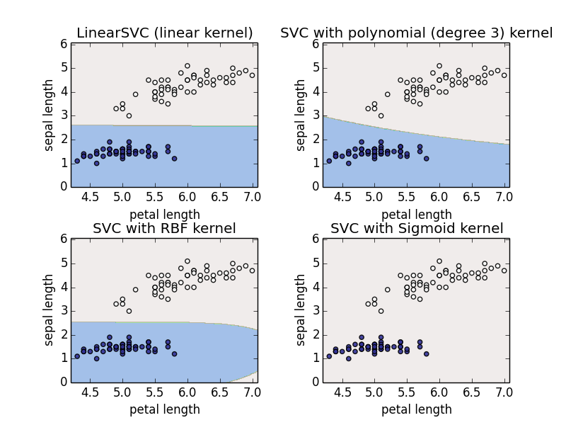
###3. Using SVM in your work. There is a package named scikit-learn in Python. Find information to install it at here. We can use the official date sets of scikit-learn, and examine the performance of classification. Here, we use Iris dataset. There are 3 kinds of iris, each sample has 4 properties which include petal length, petal width, sepal length, and sepal width.

In this experiment, we will show how to conduct a binary classification task. We removed one kind of iris, and two groups of iris are left. After this process, we have two kinds of iris, and each kind has 50 samples. And in order to draw two-dimensional chart, two properties are left: petal length and sepal length.

####3.1 Handle the dataset

#acquire and handle dataset.
from sklearn import datasets 
iris=datasets.load_iris()
dateset_property=[]
dateset_target=[]
for num in range(len(iris.target)):
    if iris.target[num]!=2: #iris.target[num]=2 is corresponding to the third kind of iris
        dateset_property.append(iris.data[num])
        dateset_target.append(iris.target[num])
x = np.array(dateset_property)
y = np.array(dateset_target)

####3.2 Train the model. In this experiment, I apply 4 kinds of kernel function, including linear,poly,RBF and sigmoid.

import numpy as np
from sklearn import svm
from sklearn.cross_validation import train_test_split

#split the dataset, and rearrange the list
x_train, x_test, y_train, y_test = train_test_split(x, y, test_size = 0.0)

# create a mesh to plot in
x_min, x_max = x_train[:, 0].min() - 0.1, x_train[:, 0].max() + 0.1
y_min, y_max = x_train[:, 1].min() - 1, x_train[:, 1].max() + 1
xx, yy = np.meshgrid(np.arange(x_min, x_max, 0.02), np.arange(y_min, y_max, 0.02))

# title for the plots
titles = ['LinearSVC (linear kernel)','SVC with polynomial (degree 3) kernel', 'SVC with RBF kernel', 'SVC with Sigmoid kernel']
clf_linear  = svm.SVC(kernel='linear').fit(x_train, y_train)
clf_poly    = svm.SVC(kernel='poly', degree=3).fit(x_train, y_train)
clf_rbf     = svm.SVC().fit(x_train, y_train)
clf_sigmoid = svm.SVC(kernel='sigmoid').fit(x_train, y_train)

####3.3 Draw plot

import matplotlib.pyplot as plt
for i, clf in enumerate((clf_linear, clf_poly, clf_rbf, clf_sigmoid)):
    #result are the predict result of all the meshgrid.
    result = clf.predict(np.c_[xx.ravel(), yy.ravel()])

    #set the composition of plot
    plt.subplot(2, 2, i + 1)
    plt.subplots_adjust(wspace=0.35, hspace=0.35)

    # Put the result into a color plot.
    z = result.reshape(xx.shape)
    plt.contourf(xx, yy, z, cmap='terrain', alpha=0.4)

    # Plot the training points
    plt.scatter(x_train[:, 0], x_train[:, 1], c=y_train, cmap='terrain',alpha=0.9)
    plt.xlabel(u'petal length')
    plt.ylabel(u'sepal length')
    plt.xlim(xx.min(), xx.max())
    plt.ylim(yy.min(), yy.max())
    plt.title(titles[i])
plt.show()

Result of classification

Reference

1. Andrew R. Webb and Keith D. Copsey Statistical Pattern Recognition(Third Edition).
2. Martin Law A Simple Introduction to Support Vector Machines.
3. Andrew Ng Machine Learning (Stanford CS229).