神经网络定义及实现

    随着GPU等硬件的引入以及其在分布式计算的应用(CUDA)，深度学习越来越得到人们的关注，但是“深度”的增加带来的问题，不是仅仅通过计算资源的提高就能解决的，一个主要的问题就是深度的增加会带来梯度弥散，以往的反向传播的训练方式不再那么有效。
    在这种情况下，主要有两种方式来训练“深度”网络，一种是进行“权共享(weights sharing)”,比如我们本文介绍的CNN(Convolutional Neural Network)就是这样;另一种解决方式就是使用限制Boltzmann机,进行逐层无监督训练，最后使用反向传播算法进行整个系统的微调。
    CNN在图像特征提取发挥着有效作用，RNN(Recurrent Neural Network)则在自然语言领域同样展现了显著的有效性。在这篇文章中，将介绍并训练一个CNN模型，之后将介绍RNN和LSTM.

0.Multi-Level Perceptron

多层感知器是最基本形式的神经网络，其由输入层、隐层和输出层组成。虽然使用Keras等高度封装的包可以使用短短几句代码完成MLP的构造，这里我们仍使用Theano(TensorFlow和Keras都是基于Theano框架的)来Step-by-Step地构建MLP，以便加深对模型的理解。

(1)首先我们构建更新方程，这里以同时考虑了更新率和梯度两方面优化的更新方程Adadelta为例：我们知道AdaGrad改进了学习速度，其为所有历史梯度的平方和，因此随着学习进行，学习速率是逐渐下降的，而Adadelta则部分保留新产生的梯度平方和。

$r = \rho \times r + (1-\rho)(d(\theta_{i-1}))^2\\ update = \frac{\sqrt{dr + \epsilon}}{\sqrt{r + \epsilon}}d(\theta_{i-1})\\ \theta_{i} = \theta_{i-1} - \lambda\times update\\ dr = \rho \times dr + (1-\rho)(update)^2$

使用Theano中的Share Variable来定义变量，该变量会在执行theano.function的updates参数中实现更新。

import theano
import theano.tensor as T
import numpy as np

def adadelta(cost, params, lr, rho):
	gparams = T.grad(cost, params)
	updates = []
	epsilon = 1e-5
	accs = [theano.shared(value=np.zeros_like(p.get_value()).astype(theano.config.
floatX)) for p in params]
	delat_accs = [theano.shared(value=np.zeros_like(p.get_value()).astype(theano.
config.floatX)) for p in params]
	for param, gparam, acc, delta_acc in zip(params, gparams, accs, delat_accs):
		acc_new = rho*acc + (1-rho)* (gparam**2)
		update = gparam*T.sqrt(delta_acc+epsilon)/T.sqrt(acc_new+epsilon)
		param_new = param - lr*update
		delta_acc_new = rho*delta_acc + (1-rho)*(update**2)
		updates.append((acc, acc_new))
		updates.append((param, param_new))
		updates.append((delta_acc, delta_acc_new))
	return updates

(2).定义MLP模型的基本参数，以及在后续构建模型所需要的cost, update以及error。

class HiddenLayer:
	def __init__(self, input, n_input, n_output, W=None, b=None, activation=T.nnet.relu):
		self.input = input
		self.n_input = n_input
		self.n_output = n_output
		if not W:
			W = np.random.uniform(low = -np.sqrt(6.0/(n_input+n_output)), high = np.sqrt(6.0/(n_input+n_output)), size = (n_input, n_output)).astype(theano.config.floatX)
		self.W = theano.shared(value=W, name='W', borrow=True)
		if not b:
			b = np.zeros(shape = (n_output,)).astype(theano.config.floatX)
		self.b = theano.shared(value=b, name='b', borrow=True)
		self.params = [self.W, self.b]
		self.output = activation(T.dot(input, self.W)+self.b)


class SoftmaxLayer:
	def __init__(self, input, n_input, n_output):
		self.input = input
		self.n_input = n_input
		self.n_output = n_output

		self.W = theano.shared(value=np.zeros(shape=(n_input, n_output)).astype(theano.config.floatX), name='W', borrow=True)
		self.b = theano.shared(value=np.zeros(shape=(n_output, )).astype(theano.config.floatX), name='b', borrow=True)

		self.params = [self.W, self.b]

		self.p_y_given_x = T.nnet.softmax(T.dot(self.input, self.W)+self.b)

		self.p_pred = T.argmax(self.p_y_given_x, axis=1)

	def cross_entropy(self, y):
		return -T.mean(T.log(self.p_y_given_x)[T.arange(y.shape[0]), y])

	def error_rate(self, y):
		return T.mean(T.neq(self.p_pred, y))


class MLP:
	def __init__(self, input, n_input, n_hiddens, n_output, activation=T.nnet.relu):
		self.input = input
		self.n_input = n_input
		self.n_output = n_output
		self.n_hiddens = n_hiddens

		layers = [n_input] + n_hiddens + [n_output]
		self.hidden_layers = []
		weight_matrix_size = zip(layers[:-1], layers[1:])
		data = input
		for n_in, n_out in weight_matrix_size[:-1]:
			self.hidden_layers.append(HiddenLayer(data, n_in, n_out))
			data = self.hidden_layers[-1].output
		n_in, n_out = weight_matrix_size[-1]
		self.output_layer = SoftmaxLayer(data, n_in, n_out)

		self.params = []
		for hidden in self.hidden_layers:
			self.params = self.params + hidden.params
		self.params = self.params + self.output_layer.params

	def get_cost_updates(self, y, lr, reg, optimizer_fun):
		cost = self.output_layer.cross_entropy(y)
		L = 0.0
		for hidden in self.hidden_layers:
			L += (hidden.W**2).sum()
		L += (self.output_layer.W**2).sum()
		cost += reg*L
		updates = optimizer_fun(cost, self.params, lr)
		return (cost, updates)
	def error_rate(self, y):
		return self.output_layer.error_rate(y)

(3) 搭建Theano计算图模型。

train_x, train_y
test_x, test_y

train_set_size, input_n = train_x.shape
test_set_size, _ = test_x.shape

# place holder
x = T.matrix('x').astype(theano.config.floatX)
y = T.ivector('y')

lr = T.scalar('lr', dtype=theano.config.floatX)
reg = T.scalar('reg', dtype=theano.config.floatX)

batch_size = 100
n_train_batch = train_set_size // batch_size
n_test_batch = test_set_size // batch_size

output_n = 10
model = MLP(x, input_n, [1000, 1000], output_n)
cost, updates = model.get_cost_updates(y, lr, reg, adadelta)

train_model = theano.function(inputs=[x, y, lr, reg], outputs = cost, updates=updates)
train_error = theano.function(inputs=[x, y, lr, reg], outputs = model.error_rate(y), on_unused_input='ignore')
test_error = theano.function(inputs=[x, y, lr, reg], outputs = model.error_rate(y), on_unused_input='ignore')

idx = np.arange(train_set_size)
for epoch in range(500):
	np.random.shuffle(idx)
	new_train_x = [train_x[i] for i in idx]
	new_train_y = [train_y[i] for i in idx]
	for batch_index in range(n_train_batch):
		train_model(new_train_x[batch_index*batch_size:(batch_index+1)*batch_size],
		new_train_y[batch_index*batch_size:(batch_index+1)*batch_size],
		0.1, 0.0)
	test_errors = [test_error(test_x[n_test_index*batch_size:(n_test_index+1)*batch_size], test_y[n_test_index*batch_size:(n_test_index+1)*batch_size], 0.1, 0.0) for n_test_index in range(n_test_batch)]

如果使用Keras定义相同的MLP模型，仅需要下属几行代码便可以完成上述所有功能。

from keras.models import Sequential
from keras.layers import Dense
from keras.optimizers import Adadelta
import keras
from utls import load_cifar10

train_x, train_y = load_cifar10('./cifar10/train/')
test_x, test_y = load_cifar10('./cifar10/test/')

train_x = train_x/255.0
test_x = test_x/255.0

train_y = keras.utils.to_categorical(train_y, 10)
test_y = keras.utils.to_categorical(test_y, 10)

model = Sequential()

model.add(Dense(1000, activation='relu', input_dim=train_x.shape[1]))
model.add(Dense(1000, activation='relu'))
model.add(Dense(10, activation='softmax'))

optimizer = Adadelta(lr=0.1, rho=0.95, epsilon=1e-5, decay=0.0)
model.compile(loss='categorical_crossentropy',
              optimizer=optimizer,
              metrics=['accuracy'])
model.fit(train_x, train_y,
          epochs=30,
          batch_size=100)
score = model.evaluate(test_x, test_y, batch_size=100)

1.Convolutional Neural Network

从仿生学的角度思考，我们获取图像时，是由一系列的神经元网络状连接而成，从串联的角度是由一系列由低级神经元（获取图像基本的像素信息）到高级神经元（抽象能力逐步增强），从并联的角度，在低级神经元层，横向来看又有无数低级神经元连接而成，这些神经元负责不同的图像采集区域。由这些低级神经元和高级神经元共同组成cnn的conv layer。而从“视网膜”，到“中枢组织”再到“大脑的视觉皮层（又分为初级高级）”相当于由若干的conv layer，这样就组成了信息逐层处理的cnn。

2.Recurrent Neural Network

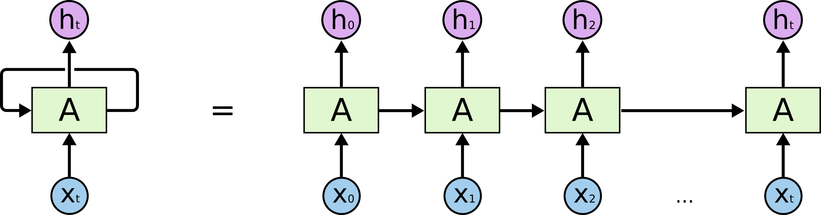
无论是卷积神经网络(cnn)还是全连接神经网络(fully connected network), forward过程中，隐层中每一层的输入都是仅来自上一层，信息是逐层传递的，但我们体验文本阅读时，上下文的关联相比与图像识别的需求更高了。我们理解一个词的含义时，不仅不要这个词本身(一个词本身也是具有许多种含义的)，同时需要来自上下文的支持，因此修正之前神经网络模型的仅从上一层获取输入，增加本层间信息流的输入，就产生了循环神经网络(recurrent nn, 后文中rnn特指recurrent nn, 而非recursive nn),接下来我将介绍一种特殊的RNN：LSTM.

3.Long Short Term Memory

一方面，较长的语句中，前后句间的word间隔过远，信息保留较少，比如：“云在‘天空’中”，‘天空’这个词很容易通过‘云’这个词来锁定，RNN对该情形也能较好地覆盖；但“我生活在法国，所以说一口流利的’法语‘”中，法语与法国间隔较远，存在明显的gap，如果关联词间的gap较大，RNN已经不能有效地关联相关信息.所以RNN只能较好地处理“short term”的情形。
另一方面,由于RNN自身结构的原因(大量的weights),较小的weights经常造成梯度弥散现象(gradient vanishing),梯度弥散现象进一步加剧了‘long term memory’的难度，较大的weights则会造成gradient exploding。

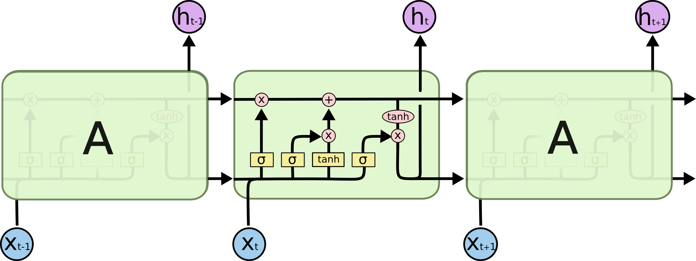
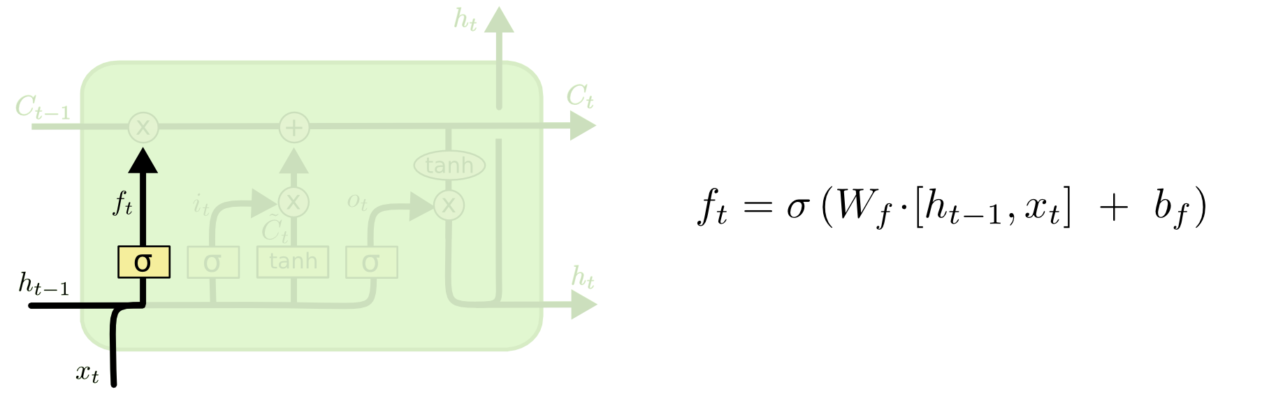
这里于是引入LSTM的概念，首先，从层内的横向角度来看，区别于RNN中横向传来的一个 $h_{t-1}$ ，这里增加一个横向传递的变量cell state: $C_{t-1}$ ，用以“线性”地保留上文信息(在传统RNN中 $wh_{t-1}*h_{t-1}＋ wx_{t}*x_{t}$ 经过一个激活函数的非线性变换为 $h_{t}$ )。

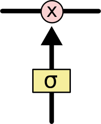
接下来是gates的概念，通过设置引入激活函数(sigmoid)来建立“门”，从而决定是否保留该项信息。每一个图中的黄色方块都是一个完整的神经元，包括weight，输入以及激活函数。激活函数(取 $\sigma(wh_{t-1}*h_{t-1}＋ wx_{t}*x_{t})$ )的结果为1时， $C_{t-1}*1$ 运算的结果即为保留之前的信息。

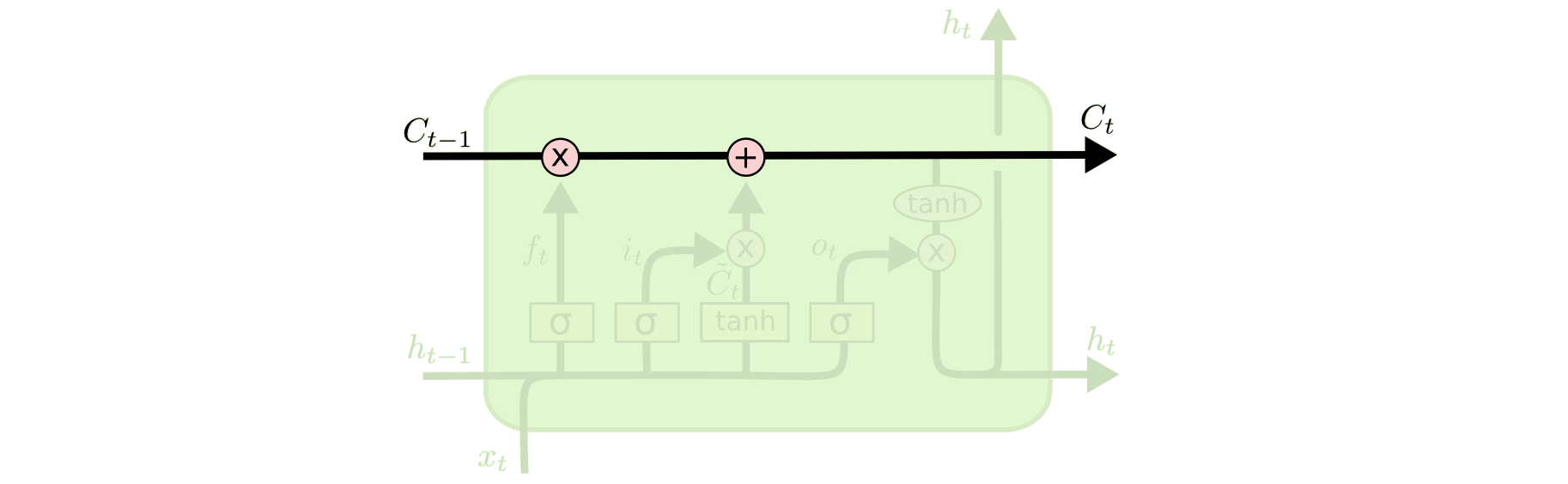
下图所示的第一个gate，是用来决定之前的信息是否舍弃的。

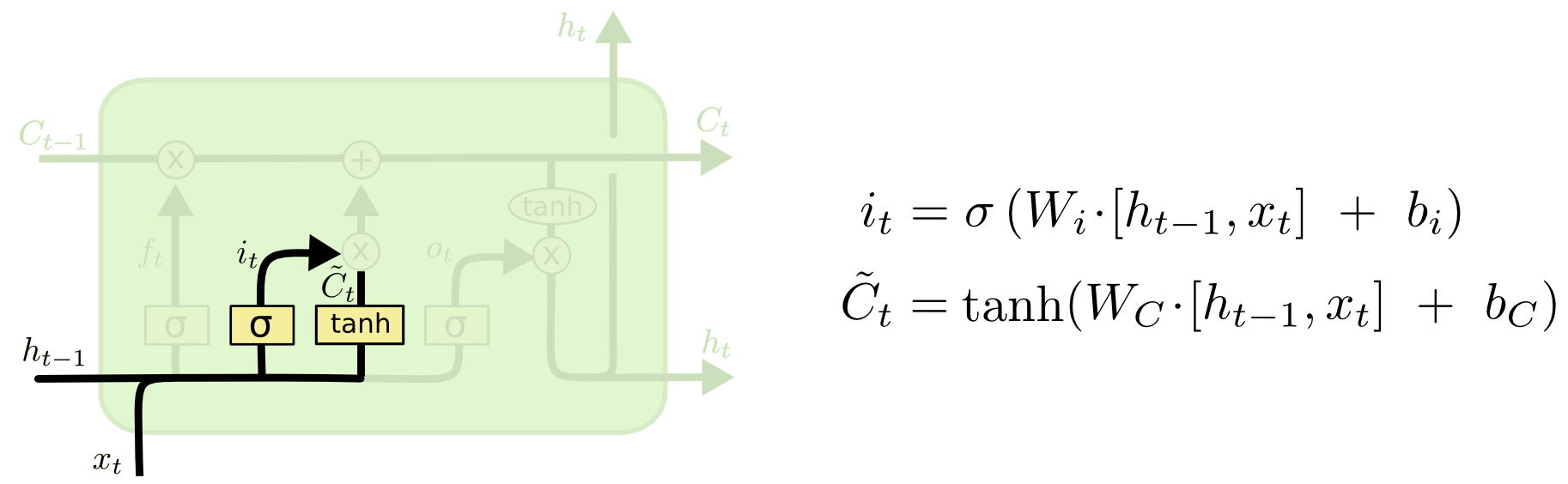
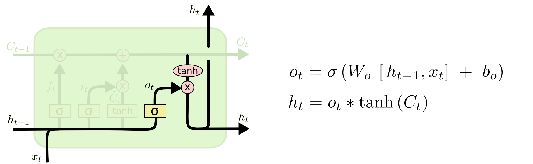
接下来我们来决定什么新信息要被加入到 $C_{t}$ 中，经过 $+$ 运算 $C_{t-1}$ 就变成了 $C_{t}$ ( $C_{t}=f_{t}*C_{t-1}+i_{t}*\hat{C}{t}$ )

剩下要输出的便是我们传递给下一隐层和同一层下一个LSTM单元的输入 $h_{t}$

3. Implement of LSTM

这里我们以Language Model为例使用Tensorflow来介绍LSTM的使用。 Language Model是NLP领域经常要用到的Model，比如将语音专为文本的应用场景下，常常会评估一个句子出现的概率，比如说“我今天吃了肯德基”这句话的概率应该比“肯德基今天吃了我”要大。为了做到这种概率的评估，一种常见的方式是给出前面几个字，我们要估计下一个单词出现在这里的概率。
下面以单词”hihello”为例，给出”hihell”为input，我们要让对应输出”ihello”的概率最大。

import tensorflow as tf
import numpy as np

# input: hihell
idx2char = ['h', 'i', 'e', 'l', 'o']
x_one_hot = [[[1,0,0,0,0],  # h 0
              [0,1,0,0,0],  # i 1
              [1,0,0,0,0],  # h 0
              [0,0,1,0,0],  # e 2
              [0,0,0,1,0],  # l 3
              [0,0,0,1,0]]] # l 3
# output: ihello
y_data = [[1, 0, 2, 3, 3, 4]] # ihello

num_classes = 5
input_dim = 5  # one-hot size
hidden_size = 5  # output from the LSTM. 5 to directly predict one-hot
batch_size = 1   # one sentence
sequence_length = 6  # |ihello| == 6
learning_rate = 0.1

X = tf.placeholder(tf.float32, [None, sequence_length, input_dim])
Y = tf.placeholder(tf.int32, [None, sequence_length])


# Feed to RNN
cell = tf.contrib.rnn.BasicLSTMCell(num_units=hidden_size, state_is_tuple=True, activation=tf.nn.relu)
initial_state = cell.zero_state(batch_size, tf.float32)
outputs, _states = tf.nn.dynamic_rnn(cell, X, initial_state=initial_state, dtype=tf.float32)

# FC layer
X_for_fc = tf.reshape(outputs, [-1, hidden_size])
# outputs = tf.contrib.layers.fully_connected(
#     inputs=X_for_fc, num_outputs=num_classes, activation_fn=None)
softmax_w = tf.get_variable("softmax_w", [hidden_size, num_classes])
softmax_b = tf.get_variable("softmax_b",[num_classes])
outputs = tf.matmul(X_for_fc, softmax_w) + softmax_b

# reshape out for sequence_loss
outputs = tf.reshape(outputs, [batch_size, sequence_length, num_classes])

weights = tf.ones([batch_size, sequence_length])
sequence_loss = tf.contrib.seq2seq.sequence_loss(logits=outputs, targets=Y, weights=weights)
loss = tf.reduce_mean(sequence_loss)
optimizer = tf.train.AdamOptimizer(learning_rate=0.1).minimize(loss)
prediction = tf.argmax(outputs, axis=2)

with tf.Session() as sess:
    sess.run(tf.global_variables_initializer())
    for i in range(2000):
        l, _ = sess.run([loss, optimizer], feed_dict={X:x_one_hot, Y:y_data})
        outputs_, result_ = sess.run([outputs, prediction], feed_dict={X:x_one_hot})
        if i%100==0:
            print(i, "loss: ", l, "outputs: ",outputs_, "prediction: ", result_, "true Y:", y_data)
            result_str = [idx2char[c] for c in np.squeeze(result_)]
            print("\tPrediction str:", ''.join(result_str))

Reference

Christopher Olah colah’s blog
Tensorflow Recurrent Neural Networks